Usage Example
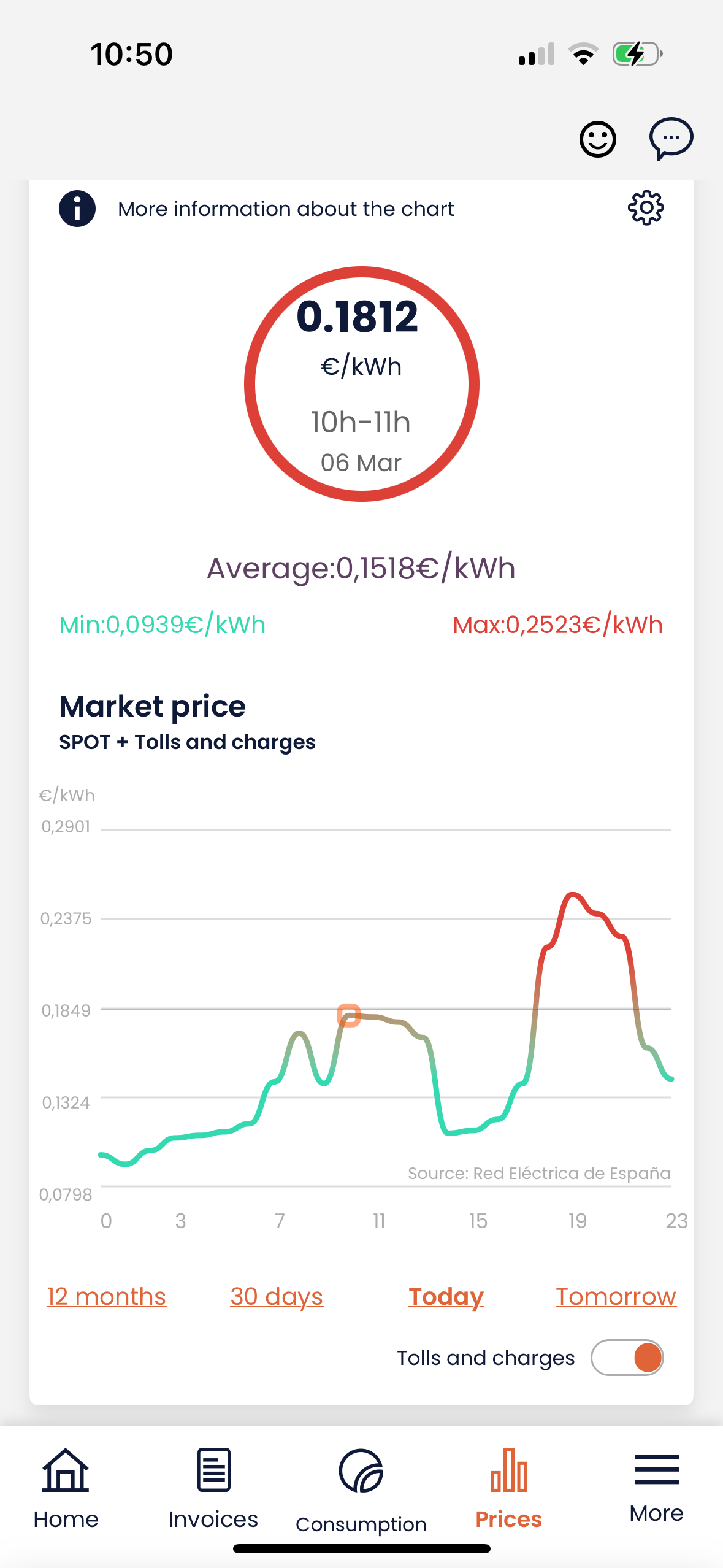
The idea for the Strom project came from realizing the huge energy price fluctuations in Spain. Since heating has a bit of flexibility, on which time you turn it on, there is an opportunity to pick the optimal hours and lower the energy bill.
Proof of Concept Hackathon
Over a weekend in January 2025 we worked on the main code for Strom. We got the code to work and interact correctly with the smart plug that we bought. Despite there being a lot of room for improvement, we celebrated this first “minimum viable setup” achievement. To iterate on
Case study
We modeled a house as a coupled, two-component system: the indoor air inside the house and its insulated wall.
The rate at which the indoor temperature drops depends on both the heat contained in the air (its heat capacity, C_air) and the ease with which heat is exchanged with the wall (its thermal resistance, R_interior). The isolated wall has its own heat capacity (C_wall) and thermal resistance (R_exterior).
The electricity price paid by private consumers roughly follows the day-ahead market price, which can be fetched through an open API. However, it typically has a minimum cost that does not reach zero, even if the overall day-ahead price does. We include this tax floor as a variable parameter, P_base, in our model.
The thermal parameters of the house were taken from Michael de Podesta’s great blog post, which can be found here.
| Parameter | Value | Units | Description |
|---|---|---|---|
C_air |
0.56 | kWh/°C | Heat capacity of indoor air |
C_wall |
3.5 | kWh/°C | Heat capacity of the insulated wall |
R_interior |
1.0 | °C/kW | Thermal resistance between air and wall |
R_exterior |
6.06 | °C/kW | Thermal resistance between wall and outside |
T_min |
18.0 | °C | Minimum allowed indoor temperature |
T_max |
24.0 | °C | Maximum allowed indoor temperature |
T_interior_init |
18.5 | °C | Initial indoor temperature |
T_wall_init |
20.0 | °C | Initial wall temperature |
Q_heater |
2.0 | kW | Power of the heating unit |
P_base |
0.01 | €/kWh | Estimated base price from the provider |
The wall acts as a thermal battery, and a smart heating pattern can charge it.
We compare two scenarios:
- A base case with a constant thermostat set to the target temperature
T_target. This is calculated as the weekly average temperature and clipped to be within the comfort temperature - An electricity cost-optimized case, where heating is scheduled based on forecasted electricity prices. Both scenarios are restricted to operate within the temperature range of
[T_min, T_max].
We coose a series of illustrative historical timeframes to show the properties of the optimized policy.
Historical analysis
25th of November
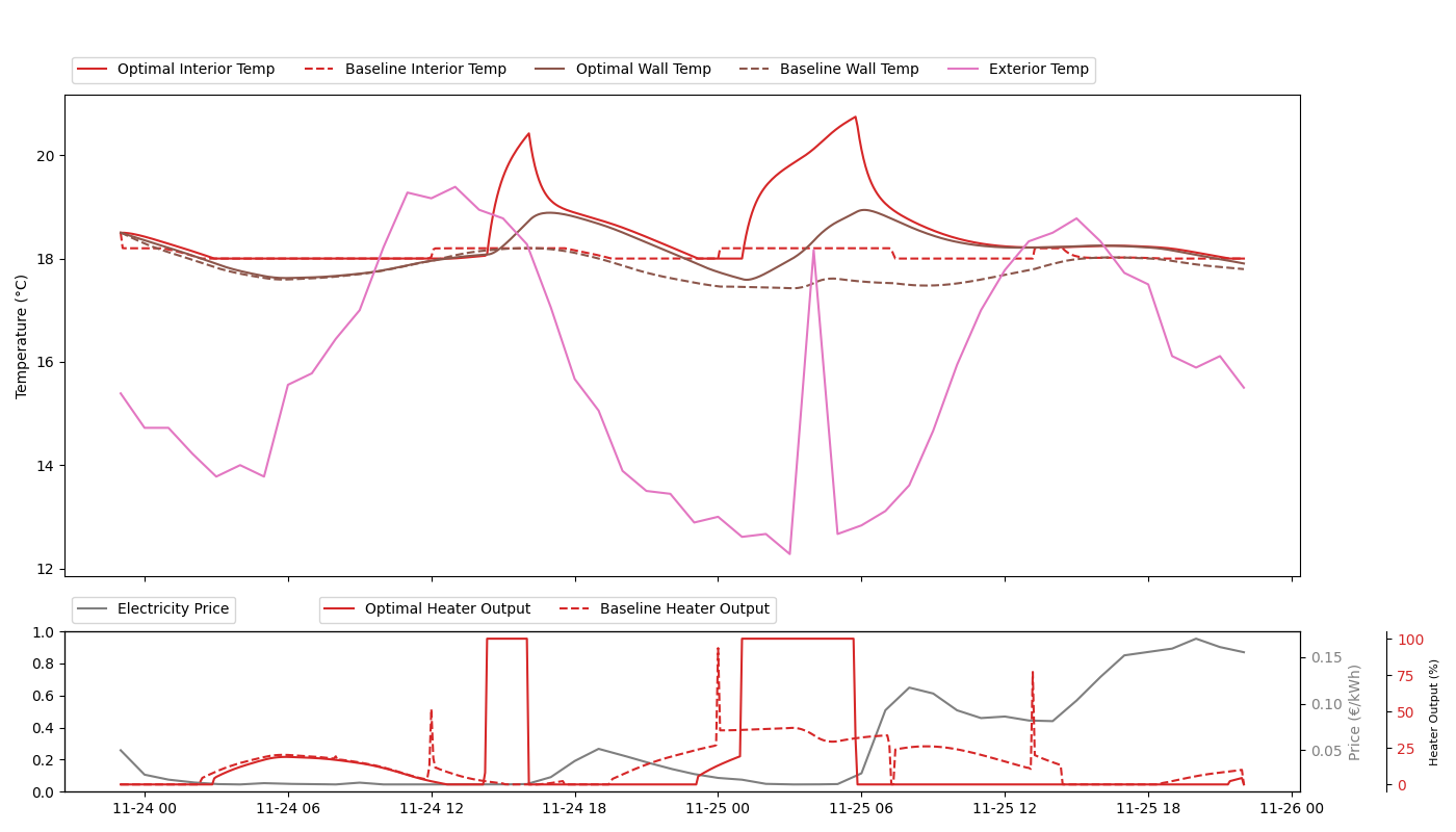
The graph shows the fluctuations in outdoor temperature and their impact on the rate of cooling of the wall and interior. It demonstrates the counteracting effects of heating the home interior on the wall. This process heats up the wall, slowing the later cooling of the interior, as the interior temperature falls only to the wall’s elevated afternoon temperature.
The cost-aware strategy heats the interior during the central portion of the day and at night, taking advantage of the daily “duck curve” energy oversupply. This approach yields significant cost savings of at least 10%, which can be further reduced with good insulation and a low minimum daily price.
The temperature dynamics of the two-lump model for this spike show that temperature first rises fast. When the temperature difference between the indoor environment and wall reaches 1°C, the heat flow into the wall is large enough to cause a significant increase in wall temperature. This maintains the temperature difference.
Once the heater is turned off, the interior temperature rapidly decreases to match the wall temperature, which only slowly decreases due to its large thermal mass and isolation from the outside. Additionally, we observe that fixed costs of electricity (such as taxes and tolls from the provider) significantly impact the overall cost.
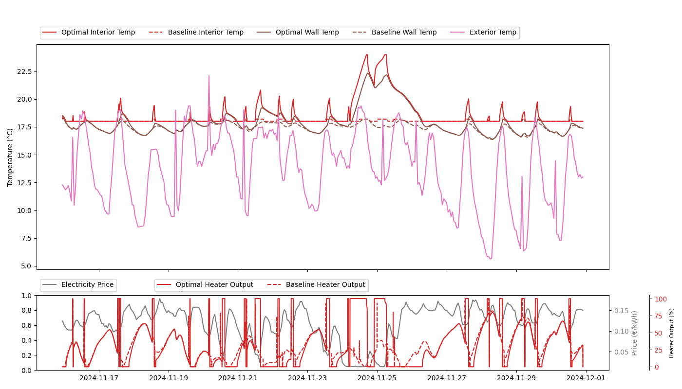
November 2024
During November 2024, we observed spikes in indoor temperature, though not limited by T_max, the upper part of the comfort zone. The system follows the expected T_min at higher energy prices like the baseline policy, which is sound cost-wise as well. The largest spike occurred on the 25th of November, a day of exceedingly low energy prices for a prolonged period of time.
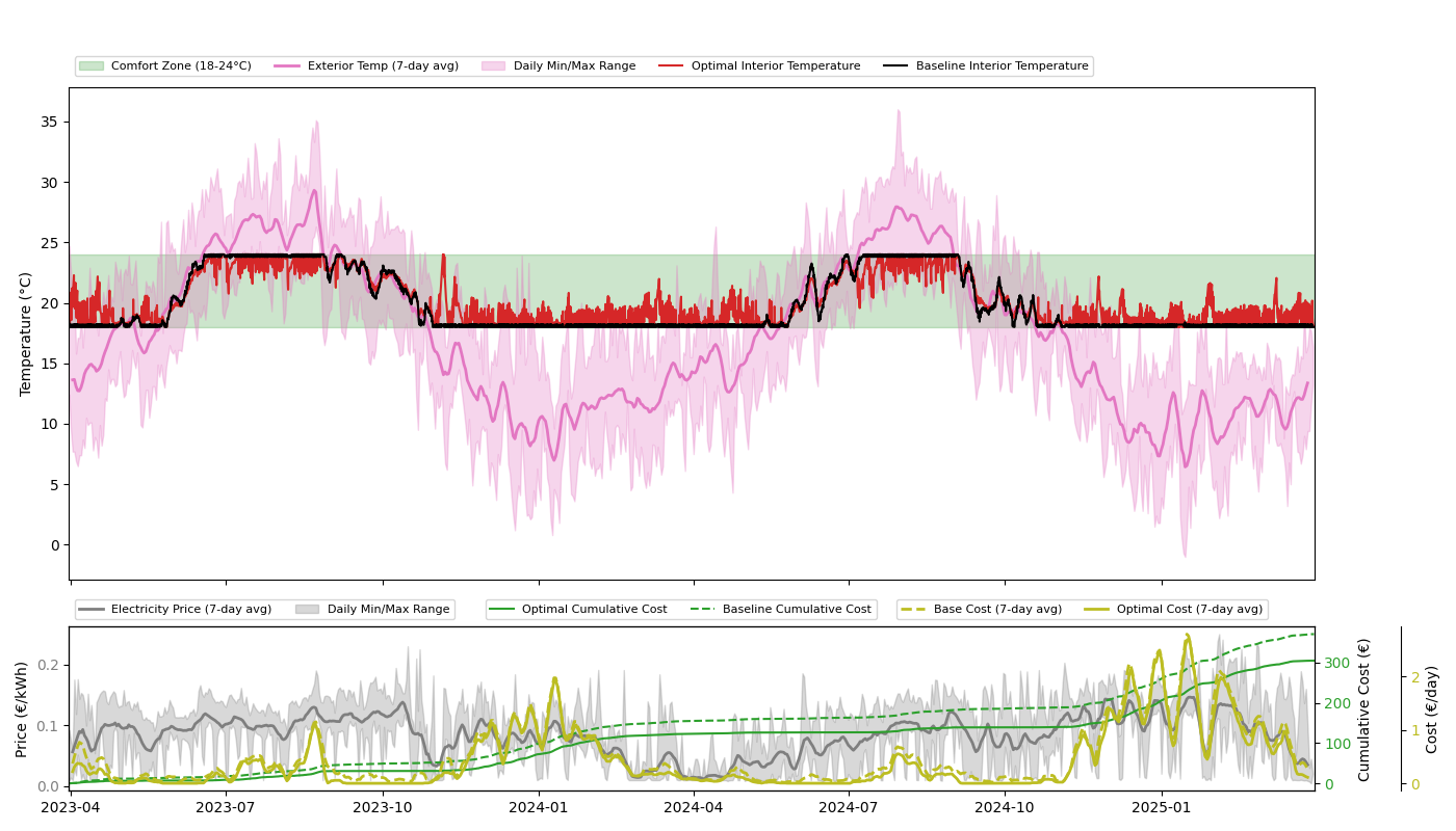
March 2023 to March 2025
For this two-year period, we added a cooling option, which is important for Barcelona where cooling costs are significant. Heating in the winter period is still the main cost driver. More realistically and efficiently, cooling can be done passively, which in our model would mean making the effective isolation parameter also controllable.
During the spring and autumn where the external temperature is on average within the comfort range, the heating and cooling costs are low. This is adequate, since it is also the time where we would also just not use neither system.
The largest differences in daily cost between the baseline policy and the cost-optimal one occur in periods where average electricity price is not too low, but still has regular minima that allow for advantageous thermal energy charging, see October 2023.
Temperature of the optimal model has many spikes as shown in the previous graphs, but they always contribute to making the temperature more comfortable in the winter and summer. The cumulative difference over the two-year period was 66€, 17% relative to the total cost of the base policy.
Upcoming improvements
Modeling
The model still lacks some additions to make it more realistic. We did not incorporate efficiency parameters. We set the base price to a low 1ct/kWh, as we intended to simulate. The insulation and thermal mass parameters are taken from a family home located in northern Europe, different values might apply in other locations.
Even at this level of detail, a factor analysis would be interesting to map out the potential savings from this method depending on location and thermal parameters.
Dedicated hardware
In order to reliably send updated instructions to the smart plug, we plan to containerize our implementation to make it executable on low-end hardware for home assistants.